'qqline' adds a line to a normal quantile-quantile plot which passes through the first and third quartiles. For good normal distribution data, the plot figure should like below.

The order for cleaning and normalization method.
For FGA, the normalization method is a big issue. So far, the method has been kept updating. "Cleaning before normalization" means normalization factor was calculated after all bad spots (defined by your cleaning settings) were removed. "Normalization after cleaning" was just reversed this order.
Attention: in "Normalization after cleaning", there was one more option "Normalize by all the spots with SNR more than" than "Normalization before cleaning".
To determine which kinds flagged spots you want to remove.
In microarray image processing software (Imagene), it would automatically mark some spots as 2,3 and et al.
Attention: in Imagene, it would automatically flag the spots with SNR<2.0 as 2. So if you want to set SNR threhold by yourself, you should exclude 2 in this option.
Remove the spots SNR less than:
To set Signal Noise Ratio threshold.
In FGA microarray, Signal Noise Ratio (SNR) for each spot was calculated by formula:
SNR = [(signal mean value of a spot)-(background mean value of a spot)] / (background standard deviation of a spot)
Remove the spots SBR less than:
To set Signal Background Ratio threshold.
In FGA microarray, Signal Background Ratio (SBR) for each spot was calculated by formula:
SBR = (signal mean value of a spot) / (background mean value of a spot)
The factor to be used in normalization method.
In order to make data comparable, each slide needs a factor to normalize all spots values. But this factor is variable by different normalization methods. In most cases, all spots within a slide should divide this factor to get normalized data.
Normalize by all spots mean/sum signals in same slide:
To normalize data from a slide by mean or sum signals.
The normalization factor in this method is the mean or sum value of signals of certain spots. Which spots were included in this calculation depends on normalization order or cleaning settings.
Normalize by all the spots with SNR more than:
To normalize data from a slide by all spots with SNR threshold.
The normalization factor in this method is the mean value of signals of the spots with SNR more than your threhold. This option was only shown after you select "normalization after cleaning" option in normalization order.
Normalize by a certain gene in same slide:
To normalize data from a slide by a certain control gene or probe.
The normalization factor in this method is the mean value of signals of a certain control gene or probe.
Normalize by greatest mean value of replicates:
To normalize data from a slide (replicate) by greatest mean value among these replicates.
The normalization factor in this method is the ratio of one slide mean value to the greatest mean value among these replicates.
Coeffient of Variations of all raw signal intensities.
Raw signal intensity is the original spot signal value from the microarray image processing software (Imagene). All spots, no matter which were bright or weak, are included. Then for each probe, we can get a set of signal values from different slides. An individual CV of the probe can be calculated by formula:
a probe CV=(standard deviation of signal values)/(mean of signal values)
Finally, total mean or std of CVs is the mean value or standard deviation of CVs of all probes.
Coeffient of Variations of spots with signal intensities.
In this calculation, only the spots with signal intensities were included. These bright spots were determined by your cleaning settings. Then, if a probe with equal or more than 2 bright spots among replicate slides, its raw signal CV were added into final total CV, otherwise it was excluded.
Coeffient of Variations of spots with normalized signal intensities.
In this calculation, all probes were as same as Real Spots CV calculation. The only difference is all values of probes were previous normalized by your normalization settings.
Romove the out-line spots more than x sigma:
For each gene, to delete some spot values out of the range of x sigma.
Among replicate slides, some spot values are much higher or less than other spots values of the same genes, because of being contaminated or missed. We called them out-line spots or outliers.
One way to recognize them is by standard deviation (sigma). For example, if one spot more or less than 2 sigma to the average value, it means this spot belongs to this gene with 4.54% possibility.
Attention: This parameter is necessary parameter.
The maximal ratio between 2 spots is:
For some gene with only 2 spots, to determine whether it is good.
In order to remove outliers, sigma range threhold was used. However, for some genes with only 2 values, that method does not work. Thus, we employ this option to check the maximal ratio between these 2 spots. But the genes with more than 2 spots are not checked by this method.
Attention: This parameter is NOT necessary parameter.
The ratio of spots number threhold:
To check the ratio of final detected spots number to original spots number.
In FGAII microarray, there were up to 3 different probes for a gene. So it supposes there are 9 final spots in triplicate slides or 6 spots in duplicate slides. But some spots can not be detected because of experimental error or other reasons. This option can determine whether a gene is reliable or not.
Attention: This parameter is necessary parameter.
The final spots number threhold:
To check the number of final spots.
This parameter is set for determining the minimal number of final spots for a gene.
Attention: This parameter is NOT necessary parameter.
To show all kinds of data from combined table.
There are several options in the frontal list. The blank box in the middle is used to set parameters. If there are more than one parameters, please use comma to separate them.
Summary => to show the summary of this combined table. No parameter required.
Statistics => to show the statistics of overlapped and unique probes or genes among replicate slides in this combined table. You can set parameters for removing some bad spots. The order for parameters is: ratio of spots' number threhold, sigma threhold, ratio of two spot values threhold, minimal spots threhold
All data in probe order => to list original and normalized data in probe order. No parameter required.
All data in gene order => to list mean data of all genes in gene order. No parameter required.
Final probe number (x) times than original number => to list mean data of the genes meeting the ratio of spots' number threshold. One parameter required for the threhold of ratio value.
In the scape of (x)sigma => to list mean data of the genes meeting the sigma threshold. One parameter required for the threhold of sigma.
(x) times and (y) sigma => to list mean data of the genes meeting the ratio of spots' number threshold and the sigma threshold synchronously. The order of parameter is: ratio of spots' number threhold, sigma threhold.
(x) times, (y) sigma, (a) ratio and (b) num => to list mean data of the genes meeting the ratio of spots' number threshold, the sigma threshold, ratio of two spot values threhold and minimal spots threhold synchronously. The order of parameter is: ratio of spots' number threhold, sigma threhold,ratio of two spot values threhold, minimal spots threhold.
To explain the abbreviation of gene categories in FGAII.
CDEG => Carbon degradation
CFIX => Carbon fixation
DSR => Dissimilatory sulfate reductase
MET => Metal reductase
Methane => methane
methane_gen => methane generation
methane_ox => methane oxidation
NFIX => Nitrogen fixation
NIT => Nitrification
NRED => Nitrogen reductase
ORG => Organic remediation
PER => perchlorate
To perform the Shapiro-Francia test for the composite hypothesis of
normality.
The test statistic of the Shapiro-Francia test is simply the
squared correlation between the ordered sample values and the
(approximated) expected ordered quantiles from the standard
normal distribution. The p-value is computed from the formula
given by Royston (1993). By the way, the normality tests check
a given set of data for similarity to the normal distribution.
The null hypothesis is that the data set is similar to the normal
distribution, therefore a sufficiently small P-value indicates non-normal data.
Reference: Royston, P. (1993): A pocket-calculator algorithm for the
Shapiro-Francia test for non-normality: an application to
medicine. Statistics in Medicine, 12, 181-184.
Attention: the numbers must be
between 5 and 5000. Missing values are allowed.
The Lilliefors (Kolmogorov-Smirnov) test:
To perform the Lilliefors (Kolmogorov-Smirnov) test for the composite hypothesis of
normality.
The test statistic is
the maximal absolute difference between empirical and hypothetical
cumulative distribution function. The p-value is computed from the
Dallal-Wilkinson (1986) formula, which is claimed to be only
reliable when the p-value is smaller than 0.1.
References:
Dallal, G.E. and Wilkinson, L. (1986): An analytic approximation
to the distribution of Lilliefors' test for normality. The
American Statistician, 40, 294-296.
Stephens, M.A. (1974): EDF statistics for goodness of fit and some
comparisons. Journal of the American Statistical Association, 69,
730-737.
Thode Jr., H.C. (2002): Testing for Normality. Marcel Dekker, New
York.
Attention: the numbers must be
greater than 4. Missing values are allowed.
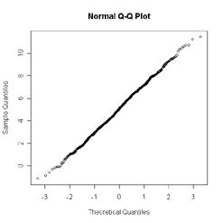
To plot the Normal porbability figure.
'qqline' adds a
line to a normal quantile-quantile plot which passes through the
first and third quartiles. For good normal distribution data, the plot figure should like below.
The quality control determination:
To determine the quality of each slides from 3 different categories.
Three categories of criteria are implemented for hybridization quality control: background level, signal level and even hybridization (spatial variation). To make the system conservative, the thresholds were set for bad hybridization.
I. Background level
1. background CV
II. Background level & Signal level
2. Average SNR
3. Average SNR of top 1000
4. SNR of 1000th signal
III. Even hybridization
5. Mantel’s r of 16S-900 genes (96 spots/array)
The decision is made based on a simple formula with multiple levels of weights on different variables (1 ~ 5). The current version is based on initial evaluation, so input from users would strengthen the system in the future.
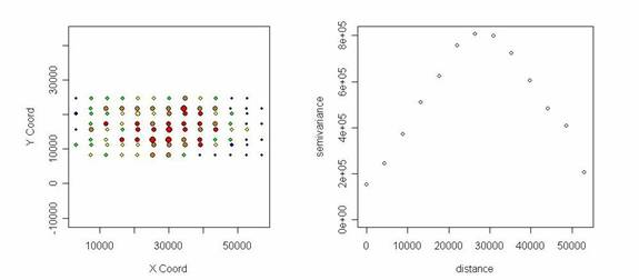
For subjective evaluation purpose, spatial map and semivariogram are provided those determined to be BAD hybridization. Size and color of dots indicate signal intensity and semivariance (y axes) is the half of the average squared difference of pairs of certain distance. Example below shows similar low signals at the both ends and higher signals in the middle of the array.